Probability explained in plain terms is the starting point for anyone who wants to make sense of data, risk, or predictions. Whether you're flipping a coin, reading a weather forecast, or interpreting survey results, probability sits at the heart of every decision involving uncertainty. For beginner data learners, the topic can feel intimidating, loaded with Greek symbols and dense formulas.
But the core ideas are surprisingly intuitive once you strip away the jargon. This guide breaks probability into four practical steps, each grounded in real examples you can apply immediately. By the end, you'll understand how to calculate basic probabilities, recognize common distributions, and avoid the mistakes that trip up most newcomers.
If you want a broader foundation, our pillar guide on statistical analysis definitions and examples covers the full landscape of analytical thinking that probability plugs into.
Key Takeaways
- Probability measures how likely an event is on a scale from zero to one.
- You only need addition and multiplication rules to solve most basic problems.
- Conditional probability changes the odds when new information arrives.
- Common distributions like normal and binomial appear constantly in real datasets.
- Misreading independent versus dependent events is the most frequent beginner mistake.
1. Understand What Probability Actually Measures
The Probability Scale
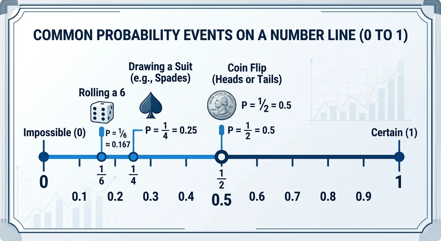
Probability assigns a number between 0 and 1 to every possible outcome. A value of 0 means the event is impossible; a value of 1 means it is certain. Everything interesting happens in between. A fair coin landing heads has a probability of 0.5, while the chance of rolling a 6 on a standard die is roughly 0.167. These numbers give you a precise, comparable way to talk about uncertainty instead of relying on vague words like "likely" or "unlikely."
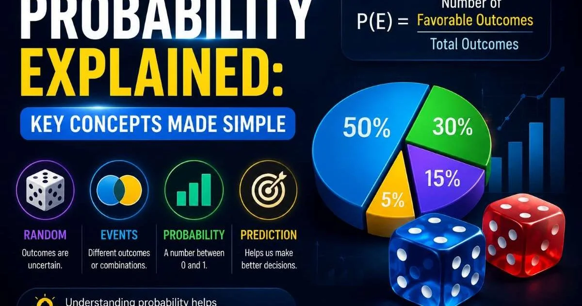
The formal definition is straightforward: probability equals the number of favorable outcomes divided by the total number of equally likely outcomes. If you draw one card from a standard 52-card deck, the probability of getting a heart is 13 divided by 52, which gives you 0.25. This classical approach works perfectly when outcomes are equally weighted. When they are not, you shift to frequency-based or subjective probability, but the beginner basics start here.
Sample Spaces and Events
A sample space is the complete set of possible outcomes for an experiment. For a single die roll, the sample space is {1, 2, 3, 4, 5, 6}. An event is any subset of that space you care about, like "rolling an even number," which is {2, 4, 6}. Defining your sample space carefully is the first real step toward accurate statistical analysis, because a sloppy sample space produces wrong answers every time.
Always write out the full sample space before calculating anything. It prevents overlooked outcomes and makes errors easy to spot.
Events can be simple (one outcome) or compound (multiple outcomes combined). The probability of a compound event depends on whether those outcomes overlap. For instance, "rolling a 2 or an even number" requires careful counting because 2 belongs to both groups. This overlap concept leads directly to the addition rule, which is the first of two core rules you need to master.
2. Learn the Two Core Rules
The Addition Rule
The addition rule handles "or" questions: what is the probability of event A or event B happening? If the two events cannot happen simultaneously (mutually exclusive), you simply add their individual probabilities. The probability of rolling a 2 or a 5 on a single die is 1/6 plus 1/6, which equals 2/6 or about 0.333. This is the simplest scenario and the one beginners should practice first.
When events overlap, you must subtract the intersection to avoid double-counting. The formula becomes P(A or B) = P(A) + P(B) minus P(A and B). Consider drawing a card that is a heart or a queen. Hearts account for 13 cards, queens account for 4, but the queen of hearts sits in both groups. So the probability is 13/52 plus 4/52 minus 1/52, giving 16/52 or about 0.308. This adjustment is where many beginners make their first mistakes.
Forgetting to subtract the overlap is the single most common error in probability homework. Double-check whether your two events share any outcomes.
The Multiplication Rule
The multiplication rule answers "and" questions: what is the probability that both A and B happen? For independent events (where one does not affect the other), multiply the probabilities directly. Flipping two coins and wanting both to show heads gives 0.5 times 0.5, equaling 0.25. Independence is the key assumption here, and verifying it matters greatly for accurate data analysis.
When events are dependent, the second probability shifts based on the first outcome. Drawing two aces from a deck without replacement is a classic example. The first ace has probability 4/52. Given that you drew an ace, only 3 aces remain among 51 cards, so the second probability is 3/51. Multiply them: (4/52) times (3/51) equals roughly 0.0045. This dependency concept bridges naturally into conditional probability, covered in the next section. Just as systematic review processes catch subtle bugs in code, careful dependency checks catch subtle errors in probability calculations.
| Feature | Addition Rule | Multiplication Rule |
|---|---|---|
| Question type | A or B? | A and B? |
| Mutually exclusive case | P(A) + P(B) | Not applicable |
| Overlapping case | P(A) + P(B) - P(A∩B) | Not applicable |
| Independent events | Not applicable | P(A) × P(B) |
| Dependent events | Not applicable | P(A) × P(B given A) |
Never multiply probabilities when events are not independent. Always ask: does knowing the first outcome change the second?
3. Apply Conditional Probability to Real Scenarios
Conditional probability measures how the likelihood of an event changes once you have additional information. Written as P(A|B), it reads "the probability of A given that B has occurred." If 60% of a company's employees use laptops and 30% use both laptops and external monitors, the probability that a laptop user also uses an external monitor is 0.30 divided by 0.60, equaling 0.50. That extra information (knowing someone uses a laptop) dramatically narrowed the field.
Probability explained through conditional thinking becomes immediately practical. Medical testing is a powerful example. Suppose a disease affects 1% of a population, and a test correctly identifies carriers 95% of the time but also gives false positives 5% of the time. Without conditional probability, you might assume a positive result is nearly certain proof of the disease. In reality, because the disease is rare, most positive results are false positives. This counterintuitive outcome surprises almost everyone who encounters it for the first time.
"A positive test result does not mean what most people think it means; conditional probability reveals why."
Bayes' Theorem in Practice
Bayes' Theorem formalizes the process of updating beliefs with new evidence. The formula is P(A|B) = [P(B|A) × P(A)] / P(B). Using the medical testing example above, you plug in the disease prevalence (prior probability), the test sensitivity, and the overall positive-test rate to find the true probability of having the disease given a positive result. For our numbers, it works out to roughly 16%, not 95%. Statistics for beginners often skip this calculation, but it is one of the most important real-world applications of probability.
Spam filters, recommendation engines, and fraud detection systems all rely on Bayesian reasoning. Each new data point updates the probability that an email is spam or a transaction is fraudulent. The logic mirrors how humans naturally revise opinions when presented with new evidence, except the math removes emotional bias from the process. Understanding Bayes' Theorem gives you a substantial advantage in chart interpretation, because you can critically evaluate whether a reported statistic accounts for base rates or ignores them entirely. Much like how identifying duplicate content requires careful attention to context, interpreting probability demands you account for all background conditions.
Whenever you see a scary-sounding statistic in the news, ask what the base rate is. That single question often changes the entire picture.
4. Recognize Common Probability Distributions
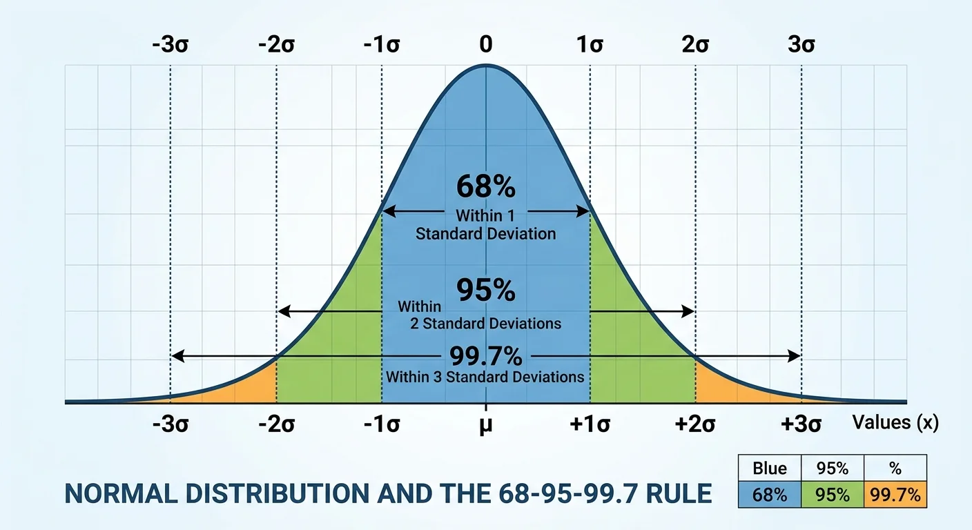
A probability distribution describes how likely each possible outcome of a random variable is. The simplest example is a uniform distribution, where every outcome has equal probability, like a fair die. In practice, data rarely follows a uniform pattern. Heights, test scores, and measurement errors typically cluster around a central value and thin out toward the extremes, forming the famous bell curve known as the normal distribution.
The binomial distribution models situations with a fixed number of independent trials, each having only two outcomes (success or failure). Flipping a coin 10 times and counting heads is a textbook binomial scenario. The Poisson distribution handles events that occur at a known average rate in a fixed interval, like the number of customer service calls per hour. Recognizing which distribution fits your data is a critical skill for any statistical analysis task, because choosing the wrong model leads to unreliable predictions.
Choosing the Right Distribution
Start by asking a few diagnostic questions. Is your variable continuous or discrete? Are there only two outcomes per trial? Is there a natural upper limit on values? These answers narrow your options quickly. Continuous data with symmetric clustering usually points to a normal distribution. Count data with no upper bound often fits Poisson. Binary trial data with a fixed count almost always calls for binomial. The probability explained through distribution choice becomes concrete once you practice matching datasets to these patterns.
Visualizing your data before picking a distribution is always worthwhile. Histograms reveal skewness and clustering patterns. Q-Q plots compare your data against a theoretical distribution. These basics of chart interpretation help you validate assumptions rather than guessing. When probability explained through the right distribution meets clean visual analysis, you get results you can actually trust and communicate to others confidently.
Frequently Asked Questions
?How do I apply the addition rule when events overlap?
?How does conditional probability differ from basic probability?
?How long does it take to understand Bayes' Theorem practically?
?What's the most common mistake when identifying independent events?
Final Thoughts
Probability is the foundation every data learner needs before tackling more advanced statistical methods. The four steps covered here, from understanding the 0-to-1 scale to recognizing distributions, give you a working toolkit for real problems.
Practice with small examples like dice, cards, and coin flips until the logic feels natural. Once conditional probability and Bayes' Theorem click, you will start noticing how often media reports and everyday claims ignore base rates. That awareness alone makes probability explained in practical terms one of the most valuable skills you can build.
Disclaimer: Portions of this content may have been generated using AI tools to enhance clarity and brevity. While reviewed by a human, independent verification is encouraged.